HP 33s User Manual
Scientific
Hide thumbs
Also See for 33s:
- Owner's manual (386 pages) ,
- User manual (9 pages) ,
- Instruction manual (7 pages)

Related Manuals for HP 33s


Summary of Contents for HP 33s
- Page 1 HP 33s scientific calculator user’s manual HP Part number F2216A-90020 Printed in China Edition 2...
- Page 2 Notice This manual and any examples contained herein are provided “as is” and are subject to change without notice. Hewlett-Packard Company makes no warranty of any kind with regard to this manual, including, but not limited to, the implied warranties of merchantability and fitness for a particular purpose.
-
Page 3: Table Of Contents
Contents Basic Operation Part 1. Getting Started Important Preliminaries............1–1 Turning the Calculator On and Off.........1–1 Adjusting Display Contrast ..........1–1 Highlights of the Keyboard and Display .......1–2 Shifted Keys..............1–2 Alpha Keys..............1–3 Cursor Keys ..............1–3 Silver Paint Keys ............1–4 Backspacing and Clearing..........1–4 Using Menus ..............1–7 Exiting Menus .............1–9 RPN and ALG Keys ...........1–10... - Page 4 Periods and Commas in Numbers........ 1–18 Number of Decimal Places ......... 1–19 SHOWing Full 12–Digit Precision........ 1–20 Fractions................ 1–21 Entering Fractions............1–21 Displaying Fractions ..........1–23 Messages ..............1–23 Calculator Memory ............1–24 Checking Available Memory ........1–24 Clearing All of Memory ..........1–24 RPN: The Automatic Memory Stack What the Stack Is .............
- Page 5 Storing Data into Variables Storing and Recalling Numbers ...........3–2 Viewing a Variable without Recalling It.........3–3 Reviewing Variables in the VAR Catalog .......3–3 Clearing Variables ............3–4 Arithmetic with Stored Variables ..........3–4 Storage Arithmetic ............3–4 Recall Arithmetic ............3–5 Exchanging x with Any Variable..........3–6 The Variable "i"...
- Page 6 Factorial ..............4–14 Gamma..............4–14 Probability ............... 4–14 Parts of Numbers ............4–16 Names of Functions............4–17 Fractions Entering Fractions ............. 5–1 Fractions in the Display............5–2 Display Rules.............. 5–2 Accuracy Indicators............. 5–3 Longer Fractions............5–4 Changing the Fraction Display..........5–4 Setting the Maximum Denominator ........
- Page 7 Editing and Clearing Equations ...........6–7 Types of Equations.............6–9 Evaluating Equations............6–9 Using ENTER for Evaluation ........6–11 Using XEQ for Evaluation ...........6–12 Responding to Equation Prompts ........6–12 The Syntax of Equations ...........6–13 Operator Precedence..........6–13 Equation Functions.............6–15 Syntax Errors ............6–18 Verifying Equations............6–18 Solving Equations Solving an Equation............7–1 Understanding and Controlling SOLVE .........7–5 Verifying the Result ............7–6...
- Page 8 Using Complex Numbers in Polar Notation......9–5 Base Conversions and Arithmetic Arithmetic in Bases 2, 8, and 16........10–2 The Representation of Numbers......... 10–4 Negative Numbers............ 10–4 Range of Numbers ............ 10–5 Windows for Long Binary Numbers ......10–6 Statistical Operations Entering Statistical Data ...........
- Page 9 Selecting a Mode............12–3 Program Boundaries (LBL and RTN) ......12–3 Using RPN, ALG and Equations in Programs....12–4 Data Input and Output ..........12–4 Entering a Program............12–5 Keys That Clear............12–6 Function Names in Programs........12–7 Running a Program............12–9 Executing a Program (XEQ).........12–9 Testing a Program............12–9 Entering and Displaying Data .........
- Page 10 Selecting a Base Mode in a Program ......12–22 Numbers Entered in Program Lines ......12–23 Polynomial Expressions and Horner's Method ....12–23 Programming Techniques Routines in Programs ............13–1 Calling Subroutines (XEQ, RTN) ........13–2 Nested Subroutines ........... 13–3 Branching (GTO) ............
- Page 11 Mathematics Programs Vector Operations ............15–1 Solutions of Simultaneous Equations ......... 15–12 Polynomial Root Finder ........... 15–20 Coordinate Transformations ..........15–32 Statistics Programs Curve Fitting..............16–1 Normal and Inverse–Normal Distributions ......16–11 Grouped Standard Deviation .......... 16–17 Miscellaneous Programs and Equations Time Value of Money ............17–1 Prime Number Generator ..........17–6 Appendixes and Reference Part 3.
- Page 12 Resetting the Calculator ............. B–2 Clearing Memory ............. B–3 The Status of Stack Lift ............B–4 Disabling Operations ..........B–4 Neutral Operations ............. B–4 The Status of the LAST X Register ......... B–6 ALG: Summary About ALG ..............C–1 Doing Two–number Arithmetic in ALG ........C–2 Simple Arithmetic ............
- Page 13 Underflow ..............D–14 More about Integration How the Integral Is Evaluated..........E–1 Conditions That Could Cause Incorrect Results ....... E–2 Conditions That Prolong Calculation Time ......E–7 Messages Operation Index Index Contents...
-
Page 15: Part 1. Basic Operation
Part 1 Basic Operation... -
Page 17: Getting Started
Getting Started Watch for this symbol in the margin. It identifies examples or keystrokes that are shown in RPN mode and must be performed differently in ALG mode. Appendix C explains how to use your calculator in ALG mode. Important Preliminaries Turning the Calculator On and Off Å... -
Page 18: Highlights Of The Keyboard And Display
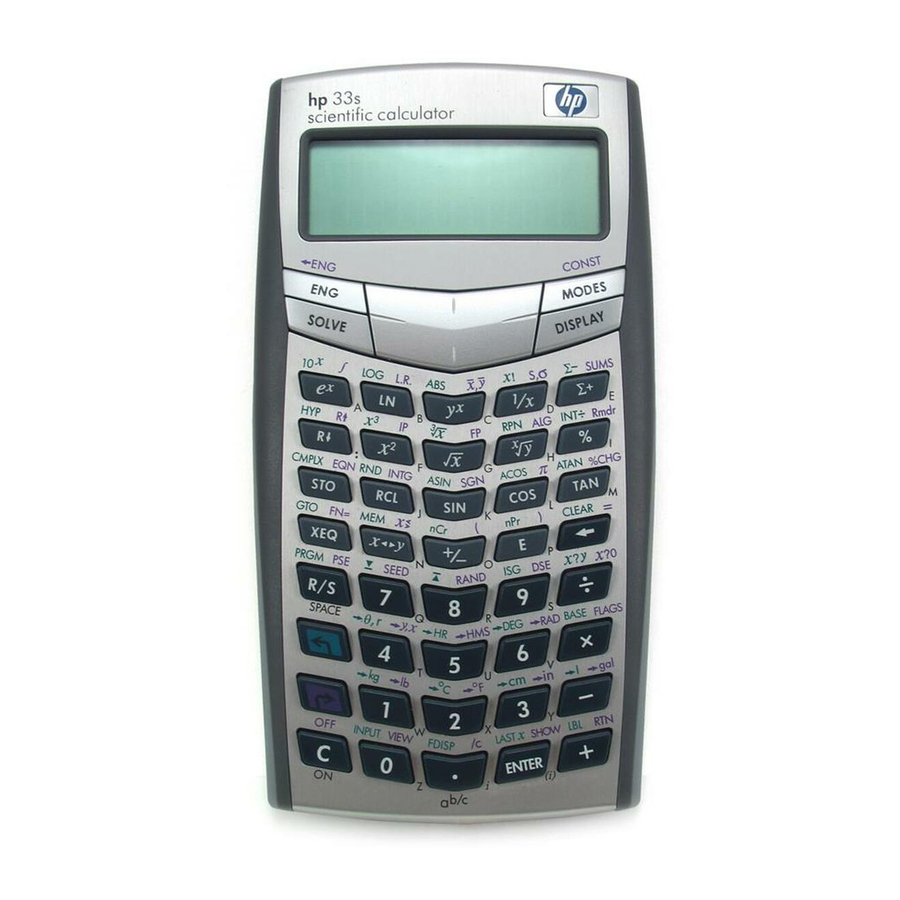
Highlights of the Keyboard and Display Shifted Keys Each key has three functions: one printed on its face, a left–shifted function (Green), and a right–shifted function (Purple). The shifted function names are ¹ printed in green and purple above each key. Press the appropriate shift key ( º... -
Page 19: Alpha Keys
¹ º ß à Pressing turns on the corresponding annunciator symbol at the top of the display. The annunciator remains on until you press the next key. To cancel a shift key (and turn off its annunciator), press the same shift key again. Alpha Keys Right-shifted Left-shifted... -
Page 20: Silver Paint Keys
Silver Paint Keys Those eight silver paint keys have their specific pressure points marked in blue position in the illustration below. To use those keys, make sure to press down the corresponding position for the desired function. Backspacing and Clearing One of the first things you need to know is how to clear: how to correct numbers, clear the display, or start over. - Page 21 Keys for Clearing Description Backspace. Keyboard–entry mode: Erases the character immediately to the left of "_" (the digit–entry cursor) or backs out of the current menu. (Menus are described in "Using Menus" on page 1–7.) If the number is completed (no cursor), clears the entire number.
- Page 22 Keys for Clearing (continued) Description The CLEAR menu ({ } { } { } { }) ¹¡ Contains options for clearing x (the number in the X–register), all variables, all of memory, or all statistical data. If you select { ...
-
Page 23: Using Menus
Using Menus There is a lot more power to the HP 33s than what you see on the keyboard. This is because 14 of the keys are menu keys. There are 14 menus in all, which provide many more functions, or more options for more functions. - Page 24 HP 33s Menus (continued) Menu Menu Chapter Name Description Other functio ns 1, 3, 12 Memory status (bytes of memory available); catalog of variables; catalog of programs (program labels). MODES 4 , 1 Angular modes and "...
-
Page 25: Exiting Menus
Example: 7 = 0.8571428571… Keys: Display: Ï ¯ Þ ({ }) Ø Õ Ï ( or Menus help you execute dozens of functions by guiding you to them with menu choices. You don't have to remember the names of the functions built into the calculator nor search through the names printed on its keyboard. -
Page 26: Rpn And Alg Keys
RPN and ALG Keys The calculator can be set to perform arithmetic operations in either RPN (Reverse Polish Notation) or ALG (Algebraic) mode. In Reverse Polish Notation (RPN) mode, the intermediate results of calculations are stored automatically; hence, you do not have to use parentheses. In algebraic (ALG) mode, you perform addition, subtraction, multiplication, and division in the traditional way. -
Page 27: The Display And Annunciators
The Display and Annunciators First Line Second Line Annunciators The display comprises two lines and annunciators. The first line can display up to 255 characters. Entries with more than 14 characters will scroll to the left. However, if entries are more than 255 characters, the characters from the 256th onward are replaced with an ellipsis ( ... - Page 28 HP 33s Annunciators Annunciator Meaning Chapter á á The " (Busy)" annunciator blinks while an operation, equation, or program is executing. ¹ When in Fraction–display mode (press É ), only one of the " " or " " halves of the "...
- Page 29 HP 33s Annunciators (continued) Annunciator Meaning Chapter Ö Õ keys are active to scroll the 1, 6 display, i.e. there are more digits to the left and right. (Equation–entry and Program–entry mode aren’t included) º Î to see the rest of a decimal number;...
-
Page 30: Keying In Numbers
Keying in Numbers You can key in a number that has up to 12 digits plus a 3–digit exponent up to â ±499. If you try to key in a number larger than this, digit entry halts and the annunciator briefly appears. If you make a mistake while keying in a number, press to backspace and Å... -
Page 31: Understanding Digit Entry
Keying in Exponents of Ten (exponent) to key in numbers multiplied by powers of ten. For example, –34 take Planck's constant, 6.6261 1. Key in the mantissa (the non–exponent part) of the number. If the mantissa is negative, press after keying in its digits. Keys: Display: 6.6261... -
Page 32: Range Of Numbers And Overflow
Keys: Display: Description: _ Digit entry not terminated: the number is not complete. If you execute a function to calculate a result, the cursor disappears because the number is complete — digit entry has been terminated. Digit entry is terminated. ... -
Page 33: One-Number Functions
One–Number Functions ¹ \ ¹ @ º To use a one–number function (such as ¹ * Ï 1. Key in the number. ( You don't need to press ¹ 2. Press the function key. (For a shifted function, press the appropriate º... -
Page 34: Controlling The Display Format
For example, To calculate: Press: Display: Ï Ù 12 + 3 Ï Ã 12 – 3 Ï ¸ Ï Ï º p Percent change from 8 to 5 Ã The order of entry is important only for non–commutative functions such as ¯... -
Page 35: Number Of Decimal Places
Number of Decimal Places All numbers are stored with 12–digit precision, but you can select the number of Þ decimal places to be displayed by pressing (the display menu). During some complicated internal calculations, the calculator uses 15–digit precision for intermediate results. -
Page 36: Showing Full 12-Digit Precision
Engineering Format ({ }) ENG format displays a number in a manner similar to scientific notation, except that the exponent is a multiple of three (there can be up to three digits before the " " or " " radix mark). This format is most useful for scientific and engineering calculations that use units specified in multiples of 10 (such as micro–, milli–, and kilo–units.) -
Page 37: Fractions
Î release Fractions The HP 33s allows you to type in and display fractions, and to perform math operations on them. Fractions are real numbers of the form a b/c where a, b, and c are integers; 0 c; and the denominator (c) must be in the range 2 through 4095. - Page 38 Ë Ë 2. Key in the fraction numerator and press again. The second separates the numerator from the denominator. Ï 3. Key in the denominator, then press or a function key to terminate digit entry. The number or result is formatted according to the current display format.
-
Page 39: Displaying Fractions
Displaying Fractions ¹ É Press to switch between Fraction–display mode and the current decimal display mode. Keys: Display: Description: Ë Ë _ Displays characters as you key them in. Ï Terminates digit entry; displays the number in the current display format. ¹... -
Page 40: Calculator Memory
Calculator Memory The HP 33s has 31KB of memory in which you can store any combination of data (variables, equations, or program lines). Checking Available Memory ¹ u Pressing displays the following menu: Where is the number of bytes of memory available. -
Page 41: Rpn: The Automatic Memory Stack
What the Stack Is Automatic storage of intermediate results is the reason that the HP 33s easily processes complex calculations, and does so without parentheses. The key to automatic storage is the automatic, RPN memory stack. -
Page 42: The X And Y-Registers Are In The Display
0.0000 "Oldest" number 0.0000 Displayed 0.0000 0.0000 Displayed The most "recent" number is in the X–register: this is the number you see in the second line of the display. In programming, the stack is used to perform calculations, to temporarily store intermediate results, to pass stored data (variables) among programs and subroutines, to accept input, and to deliver output. -
Page 43: Reviewing The Stack
Reviewing the Stack (Roll Down) < (roll down) key lets you review the entire contents of the stack by "rolling" the contents downward, one register at a time. You can see each number when it enters the X–register. Ï Ï Ï... -
Page 44: Exchanging The X- And Y-Registers In The Stack
Exchanging the X– and Y–Registers in the Stack Another key that manipulates the stack contents is (x exchange y). This key swaps the contents of the X– and Y–registers without affecting the rest of the stack. Pressing twice restores the original order of the X– and Y–register contents. function is used primarily to swap the order of numbers in a calculation. -
Page 45: How Enter Works
3. The stack drops. Notice that when the stack lifts, it replaces the contents of the T– (top) register with the contents of the Z–register, and that the former contents of the T–register are lost. You can see, therefore, that the stack's memory is limited to four numbers. -
Page 46: How Clear X Works
Using a Number Twice in a Row Ï You can use the replicating feature of to other advantages. To add a Ï Ù number to itself, press Filling the stack with a constant Ï The replicating effect of together with the replicating effect of stack drop (from T into Z) allows you to fill the stack with a numeric constant for calculations. -
Page 47: The Last X Register
During program entry, deletes the currently–displayed program line and Å cancels program entry. During digit entry, backspaces over the displayed number. Å If the display shows a labeled number (such as ), pressing cancels that display and shows the X–register. When viewing an equation, displays the cursor at the end the equation to allow for editing. -
Page 48: Correcting Mistakes With Last X
2. Reusing a number in a calculation. See appendix B for a comprehensive list of the functions that save x in the LAST X register. Correcting Mistakes with LAST X Wrong One–Number Function ¹ Í If you execute the wrong one–number function, use to retrieve the Å... -
Page 49: Reusing Numbers With Last X
Example: Suppose you made a mistake while calculating 19 = 304 There are three kinds of mistakes you could have made: Wrong Mistake: Correction: Calculation: Ï Ã ¹ Í Ù Wrong function ¹ Í ¸ Ï ¸ ¹ Í ¸ Wrong first number Ï... - Page 50 96.704 Y 96.7040 96.7040 96.7040 52.3947 52.3 947 149.0987 LAST X 52.3947 149.0987 2.8457 52.3947 LAST X 52.3947 52.3947 Keys: Display: Description: Ï 96.704 Enters first number. Ù 52.3947 Intermediate result. ¹ Í Brings back display from before Ù...
-
Page 51: Chain Calculations In Rpn Mode
(12 + 3) ... (12 + 3) = 1 5 … then you would multiply the intermediate result by 7: (15) 7 = 105 Solve the problem in the same way on the HP 33s, starting inside the parentheses: Keys: Display: Description: Ï... - Page 52 (5 + 6). Finally, you would multiply the two intermediate results to get the answer. Work through the problem the same way with the HP 33s, except that you don't have to write down intermediate answers—the calculator remembers them for you.
-
Page 53: Exercises
Exercises Calculate: 3805 0000 Solution: Ï ¸ ? ¯ 16.3805 Calculate: 5743 Solution: Ï Ù Ï Ù ¸ ? Ï Ù Ï Ù ¸ ? Ù Calculate: (10 – 5) [(17 – 12) 4] = 0.2500 Solution: Ï Ã ¸ Ï... -
Page 54: More Exercises
This method takes one additional keystroke. Notice that the first intermediate result is still the innermost parentheses (7 3). The advantage to working a problem left–to–right is that you don't have to use to reposition operands for à ¯ nomcommutaiive functions ( However, the first method (starting with the innermost parentheses) is often preferred because: It takes fewer keystrokes. - Page 55 A Solution: Ï Ù Ï Ã ¸ Ï Ã ¯ Calculate: – (13 9) + 1/7 = 412.1429 A Solution: Ï ¸ à , Ù Calculate: 5961 Solution: Ï ¸ Ï w à ¯ ? 12.5 Ï ¸ Ï Ï ) Ã...
-
Page 57: Storing Data Into Variables
Storing Data into Variables The HP 33s has 31KB of user memory: memory that you can use to store numbers, equations, and program lines. Numbers are stored in locations called variables, each named with a letter from A through Z. (You can choose the letter to remind you of what is stored there, such as B for bank balance and C for the speed of light.) -
Page 58: Storing And Recalling Numbers
Each white letter is associated with a key and a unique variable. The letter keys are automatically active when needed. (The A..Z annunciator in the display confirms this.) Note that the variables, X, Y, Z and T are different storage locations from the X–register, Y–register, Z–register, and T–register in the stack. -
Page 59: Viewing A Variable Without Recalling It
Viewing a Variable without Recalling It º È function shows you the contents of a variable without putting that number in the X–register. The display is labeled for the variable, such as: º È is most often used in programming, but it is useful anytime you want to view a variable's value without affecting the contents of t he stack. -
Page 60: Clearing Variables
Clearing Variables Variables' values are retained by Continuous Memory until you replace them or clear them. Clearing a variable stores a zero there; a value of zero takes no memory. To clear a single variable: Store zero in it: Press 0 variable. -
Page 61: Recall Arithmetic
Result: 15 that is,A Recall Arithmetic h Ù h à h ¸ h ¯ Recall arithmetic uses , or to do arithmetic in the X–register using a recalled number and to leave the result in the display. Only the X–register is affected. New x = Previous x {+, –, , } Variable For example, suppose you want to divide the number in the X–register (3, h ¯... -
Page 62: Exchanging X With Any Variable
Keys: Display: Description: Stores the assumed values into the variable. e Ù Adds1 to D, E, and F. e Ù Ù º È Displays the current value of D. º È ... -
Page 63: The Variable "I
º v Exchanges contents of the X–register and variable A. º v Exchanges contents of the X–register and variable A. The Variable "i" Ë There is a 27th variable that you can access directly — the variable i. The is labeled "i", and it means i whenever the A..Z annunciator is on. -
Page 65: Real-Number Functions
Real–Number Functions This chapter covers most of the calculator's functions that perform computations on real numbers, including some numeric functions used in programs (such as ABS, the absolute–value function): Exponential and logarithmic functions. Quotient and Remainder of Divisions. Power functions. ( Trigonometric functions. -
Page 66: Quotient And Remainder Of Division
To Calculate: Press: & Natural logarithm (base e) ¹ $ Common logarithm (base 10) Natural exponential ¹ ! Common exponential (antilogarithm) Quotient and Remainder of Division ¹ b º ` You can use to produce either the quotient or remainder of division operations involving two integers. 1. -
Page 67: Trigonometry
Ï In RPN mode, to calculate a number y raised to a power x, key in y then press . (For y > 0, x can be any number; for y < 0, x must be an odd integer; for y = 0, x must be positive.) To Calculate: Press: Result:... -
Page 68: Setting The Angular Mode
Setting the Angular Mode The angular mode specifies which unit of measure to assume for angles used in trigonometric functions. The mode does not convert numbers already present (see "Conversion Functions" later in this chapter). 360 degrees = 2 radians = 400 grads Ý... - Page 69 Example: Show that cosine (5/7) radians and cosine 128.57° are equal (to four significant digits). Keys: Display: Description: Ý { } Sets Radians mode; RAD annunciator on. Ë Ë Ï 5/7 in decimal format. º j ¸ n Cos (5/7) .
-
Page 70: Hyperbolic Functions
Hyperbolic Functions With x in the display: To Calculate: Press: ¹ : k Hyperbolic sine of x (SINH). ¹ : n Hyperbolic cosine of x (COSH). ¹ : q Hyperbolic tangent of x (TANH). ¹ : ¹ i Hyperbolic arc sine of x (ASINH). ¹... - Page 71 Ù Total cost (base price + 6% tax). Suppose that the $15.76 item cost $16.12 last year. What is the percentage change from last year's price to this year's ? Keys: Display: Description: Ï 16.12 º p 15.76 This year's price dropped about ...
-
Page 72: Physics Constants
Physics Constants º There are 40 physics constants in the CONST menu. You can press Ü to view the following items. CONST Menu Items Description Value –1 { } Speed of light in vacuum 299792458 m s –2 { } Standard acceleration of gravity 9.80665 m s –11... -
Page 73: Conversion Functions
Items Description Value –15 { } Classical electron radius 2.817940285 10 { Characteristic impendence of 376.730313461 vacuum –12 { } Compton wavelength 2.426310215 10 –15 Neutron Compton wavelength 1.319590898 10 –15 Proton Compton wavelength 1.321409847 10 ... -
Page 74: Coordinate Conversions
Coordinate Conversions , r and , r y , x . The function names for these conversions are y , x Polar coordinates ( r , ) and rectangular coordinates ( x , y ) are measured as shown in the illustration. The angle uses units set by the current angular mode. - Page 75 Example: Polar to Rectangular Conversion. In the following right triangles, find sides x and y in the triangle on the left, and hypotenuse r and angle in the triangle on the right. Keys: Display: Description: Ý { } Sets Degrees mode. ...
-
Page 76: Time Conversions
_ 36.5 77.8 ohms Keys: Display: Description: Ý { } Sets Degrees mode. z Ï 36.5 Enters , degrees of voltage lag. 77.8 _ Enters r , ohms of total impedance. º ± Calculates x , ohms resistance, R . ... -
Page 77: Angle Conversions
1. Key in the angle (in decimal degrees or radians) that you want to convert. º µ ¹ ´ 2. Press . The result is displayed. Unit Conversions The HP 33s has eight unit–conversion functions on the keyboard: ºC, ºF, gal. To Convert: Press: Displayed Results: ¹... -
Page 78: Probability Functions
Probability Functions Factorial To calculate the factorial of a displayed non-negative integer x (0 x 253), press ¹ * (the left–shifted key). Gamma To calculate the gamma function of a noninteger x , ( x ), key in ( x – 1) and press ¹... - Page 79 The RANDOM function uses a seed to generate a random number. Each random number generated becomes the seed for the next random number. Therefore, a sequence of random numbers can be repeated by starting with the same seed. You can store a new seed with the SEED function. If memory is cleared, the seed is reset to zero.
-
Page 80: Parts Of Numbers
Parts of Numbers These functions are primarily used in programming. Integer part º > To remove the fractional part of x and replace it with zeros, press . (For example, the integer part of 14.2300 is 14.0000.) Fractional part º [ To remove the integer part of x and replace it with zeros, press . -
Page 81: Names Of Functions
Names of Functions You might have noticed that the name of a function appears in the display when you press and hold the key to execute it. (The name remains displayed for as long as you hold the key down.) For instance, while pressing , the display shows ... -
Page 83: Fractions
Fractions "Fractions" in chapter 1 introduces the basics about entering, displaying, and calculating with fractions: Ë To enter a fraction, press twice — after the integer part, and between the Ë Ë numerator and denominator. To enter 2 , press 2 8. -
Page 84: Fractions In The Display
If you didn't get the same results as the example, you may have accidentally changed how fractions are displayed. (See "Changing the Fraction Display" later in this chapter.) The next topic includes more examples of valid and invalid input fractions. You can type fractions only if the number base is 10 —... -
Page 85: Accuracy Indicators
Entered Value Internal Value Displayed Fraction 2.37500000000 14.4687500000 4.50000000000 9.60000000000 2.83333333333 0.00183105469 8192 12345 12345678 (Illegal entry) â (Illegal entry) â 16384 Accuracy Indicators The accuracy of a displayed fraction is indicated by the annunciators at the right of the display. -
Page 86: Longer Fractions
This is especially important if you change the rules about how fractions are displayed. (See "Changing the Fraction Display" later.) For example, if you force all fractions to have 5 as the denominator, then is displayed as 3.3333 because the exact fraction is approximately , "a little above"... -
Page 87: Setting The Maximum Denominator
You can select one of three fraction formats. The next few topics show how to change the fraction display. Setting the Maximum Denominator For any fraction, the denominator is selected based on a value stored in the calculator. If you think of fractions as a b/c , then /c corresponds to the value that controls the denominator. -
Page 88: Examples Of Fraction Displays
To select a fraction format, you must change the states of two flags . Each flag can be "set" or "clear," and in one case the state of flag 9 doesn't matter. To Get This Fraction Format: Change These Flags: Clear —... -
Page 89: Rounding Fractions
Fraction Number Entered and Fraction Displayed Format 2.9999 Most precise 2 1/2 2 2/3 2 9/14 Factors of 2 1/2 2 11/16 2 5/8 denominator Fixed 2 0/16 2 8/16 2 11/16 3 0/16 2 10/16 denominator For a /c value of 16. Example: Suppose a stock has a current value of 48 . -
Page 90: Fractions In Equations
In an equation or program, the RND function does fractional rounding if Fraction–display mode is active. Example: Suppose you have a 56 –inch space that you want to divide into six equal sections. How wide is each section, assuming you can conveniently measure –inch increments ? What's the cumulative roundoff error ? Keys: Display:... -
Page 91: Fractions In Programs
Fractions in Programs When you're typing a program, you can type a number as a fraction — but it's converted to its decimal value. All numeric values in a program are shown as decimal values — Fraction–display mode is ignored. When you're running a program, displayed values are shown using Fraction–display mode if it's active. -
Page 93: Entering And Evaluating Equations
Entering and Evaluating Equations How You Can Use Equations You can use equations on the HP 33s in several ways: For specifying an equation to evaluate (this chapter). For specifying an equation to solve for unknown values (chapter 7). For specifying a function to integrate (chapter 8). - Page 94 Begins a new equation, turning on the " " equation–entry cursor. turns on the A..Z annunciator so you can enter a variable name. º ¢ V types and moves the cursor to the right. _ Digit entry uses the "_"...
-
Page 95: Summary Of Equation Operations
Summary of Equation Operations All equations you create are saved in the equation list. This list is visible whenever you activate Equation mode. You use certain keys to perform operations involving equations. They're described in more detail later. Operation º d Enters and leaves Equation mode. -
Page 96: Entering Equations Into The Equation List
Entering Equations into the Equation List The equation list is a collection of equations you enter. The list is saved in the calculator's memory. Each equation you enter is automatically saved in the equation list. To enter an equation: 1. Make sure the calculator is in its normal operating mode, usually with a number in the display. -
Page 97: Numbers In Equations
The cursor changes back when you press a nonnumeric key. Functions in Equations You can enter many HP 33s functions in an equation. A complete list is given under “Equation Functions” later in this chapter. Appendix G, "Operation Index,"... -
Page 98: Parentheses In Equations
Parentheses in Equations You can include parentheses in equations to control the order in which operations º y º | are performed. Press to insert parentheses. (For more information, see "Operator Precedence" later in this chapter.) Example: Entering an Equation. Enter the equation r = 2 cos ( t –... -
Page 99: Editing And Clearing Equations
if there are no equations in the equation list or if the equation pointer is at the top of the list. The current equation (the last equation you viewed). × Ø 2. Press to step through the equation list and view each equation. The list "wraps around"... - Page 100 To edit an equation you're typing: 1. Press repeatedly until you delete the unwanted number or function. If you're typing a decimal number and the "_" digit–entry cursor is on, deletes only the rightmost character. If you delete all characters in the number, the calculator switches back to the "...
-
Page 101: Types Of Equations
Å Leaves Equation mode. Types of Equations The HP 33s works with three types of equations: Equalities. The equation contains an "=", and the left side contains more than just a single variable. For example, x is an equality. - Page 102 "=" in an equation essentially treated as " – ". The value is a measure of how well the equation balances. Ï The HP 33s has two keys for evaluating equations: . Their actions differ only in how they evaluate assignment equations: returns the value of the equation, regardless of the type of equation.
-
Page 103: Using Enter For Evaluation
The evaluation of an equation takes no values from the stack — it uses only numbers in the equation and variable values. The value of the equation is returned to the X–register. The LAST X register isn't affected. Using ENTER for Evaluation Ï... -
Page 104: Using Xeq For Evaluation
¯ Changes cubic millimeters to liters (but doesn't change V ). Using XEQ for Evaluation If an equation is displayed in the equation list, you can press to evaluate the equation. The entire equation is evaluated, regardless of the type of equation. The result is returned to the X–register. -
Page 105: The Syntax Of Equations
¥ To change the number, type the new number and press . This new number writes over the old value in the X–register. You can enter a number as a fraction if you want. If you need to calculate a number, use normal ¥... - Page 106 Order Operation Example Functions and Parentheses , Power ( Unary Minus ( Multiply and Divide , Add and Subtract , Equality So, for example, all operations inside parentheses are performed before operations outside the parentheses.
-
Page 107: Equation Functions
Equation Functions The following table lists the functions that are valid in equations. Appendix G, "Operation Index" also gives this information. ALOG SQRT INTG IDIV RMDR ASIN ACOS ATAN SINH COSH TANH ASINH ACOSH ATANH %CHG XROOT CBRT Cn,r Pn,r °C °F RANDOM... - Page 108 The following equation calculates the perimeter of a trapezoid. This is how the equation might appear in a book: Perimeter = a + b + h ( The following equation obeys the syntax rules for HP 33s equations: 6–16 Entering and Evaluating Equations...
- Page 109 Parentheses used to group items P=A+B+Hx(1 SIN(T)+1 SIN(F)) ÷ ÷ Single No implied Division is done letter multiplication before addition name Th e next equation also obeys the syntax rules. This equation uses the inverse function, , instead of the fractional form, . Notice that the SIN function is "nested"...
-
Page 110: Syntax Errors
(See "Editing and Clearing Equations" earlier in this chapter.) By not checking equation syntax until evaluation, the HP 33s lets you create "equations" that might actually be messages. This is especially useful in programs, as described in chapter 12. -
Page 111: Solving Equations
Solving Equations Ï In chapter 6 you saw how you can use to find the value of the left–hand variable in an assignment –type equation. Well, you can use SOLVE to find the value of any variable in any type of equation. For example, consider the equation –... - Page 112 ¥ If the displayed value is the one you want, press ¥ If you want a different value, type or calculate the value and press (For details, see "Responding to Equation Prompts" in chapter 6.) Å ¥ You can halt a running calculation by pressing When the root is found, it's stored in the unknown variable, and the variable value is VIEWed in the display.
- Page 113 Ï Terminates the equation and displays the left end. º Î Checksum and length. g (acceleration due to gravity) is included as a variable so you can change it for different units (9.8 m/s or 32.2 ft/s Calculate how many meters an object falls in 5 seconds, starting from rest.
- Page 114 Example: Solving the Ideal Gas Law Equation. The Ideal Gas Law describes the relationship between pressure, volume, temperature, and the amount (moles) of an ideal gas: V = N where P is pressure (in atmospheres or N/m ), V is volume (in liters), N is the number of moles of gas, R is the universal gas constant (0.0821 liter–atm/mole–K or 8.314 J/mole–K), and T is temperature (Kelvins: K=°C + 273.1).
-
Page 115: Understanding And Controlling Solve
¥ Stores 297.1 in T ; solves for P in atmospheres. A 5–liter flask contains nitrogen gas. The pressure is 0.05 atmospheres when the temperature is 18°C. Calculate the density of the gas ( N 28/ V , where 28 is the molecular weight of nitrogen). -
Page 116: Verifying The Result
When SOLVE evaluates an equation, it does it the same way does — any "=" in the equation is treated as a " – ". For example, the Ideal Gas Law equation is evaluated as P V – ( N T ). -
Page 117: Interrupting A Solve Calculation
Interrupting a SOLVE Calculation Å ¥ To halt a calculation, press . The current best estimate of the root is in º È the unknown variable; use to view it without disturbing the stack. Choosing Initial Guesses for SOLVE The two initial guesses come from: The number currently stored in the unknown variable. - Page 118 If an equation does not allow certain values for the unknown, guesses can prevent these values from occurring. For example, y = t + log x results in an error if x 0 (message ). In the following example, the equation has more than one root, but guesses help find the desired root.
- Page 119 Type in the equation: Keys: Display: Description: º d Selects Equation mode º ¢ and starts the equation. º y à º | ¸ º y à h º | ¸ ¸ h Ï...
- Page 120 Keys: Display: Description: < This value from the Y–register is the estimate made just prior to the final result. Since it is the same as the solution, the solution is an exact root. < This value from the Z–register ...
-
Page 121: For More Information
For More Information This chapter gives you instructions for solving for unknowns or roots over a wide range of applications. Appendix D contains more detailed information about how the algorithm for SOLVE works, how to interpret results, what happens when no solution is found, and conditions that can cause incorrect results. -
Page 123: Integrating Equations
Integrating Equations Many problems in mathematics, science, and engineering require calculating the definite integral of a function. If the function is denoted by f(x) and the interval of integration is a to b , then the integral can be expressed mathematically as ∫... -
Page 124: Integrating Equations ( ∫ Fn)
Integrating Equations ( ∫ FN) To integrate an equation: 1. If the equation that defines the integrand's function isn't stored in the equation list, key it in (see "Entering Equations into the Equation List" in chapter 6) and leave Equation mode. The equation usually contains just an expression. Ï... - Page 125 Find the Bessel function for x– values of 2 and 3. Enter the expression that defines the integrand's function: cos ( x sin t ) Keys: Display: Description: ¹ ¡ { } Clears memory. { } º d Current equation or Selects Equation mode.
- Page 126 Now calculate J (3) with the same limits of integration. You must respecify the limits of integration (0, ) since they were pushed off the stack by the subsequent division by . Keys: Display: Description: Ï º j Enters the limits of integration ...
-
Page 127: Accuracy Of Integration
Keys: Display: Description: º d The current equation Selects Equation mode. or Starts the equation. º | The closing right parenthesis is required in this case. ¯ h Ï Terminates the equation. º Î Checksum and length. -
Page 128: Specifying Accuracy
Specifying Accuracy The display format's setting (FIX, SCI, ENG, or ALL) determines the precision of the integration calculation: the greater the number of digits displayed, the greater the precision of the calculated integral (and the greater the time required to calculate it). - Page 129 º " The integral approximated to ∫ two decimal places. The uncertainty of the approximation of the integral. The integral is 1.61±0.0161. Since the uncertainty would not affect the approximation until its third decimal place, you can consider all the displayed digits in this approximation to be accurate.
-
Page 130: For More Information
. For More Information This chapter gives you instructions for using integration in the HP 33s over a wide range of applications. Appendix E contains more detailed information about how the algorithm for integration works, conditions that could cause incorrect results and conditions that prolong calculation time, and obtaining the current approximation to an integral. -
Page 131: Operations With Complex Numbers
Ï 2. Press 3. Type the real part. Complex numbers in the HP 33s are handled by entering each part (imaginary and real) of a complex number as a separate entry. To enter two complex numbers, ¹ c you enter four separate numbers. To do a complex operation, press before the operator. -
Page 132: Complex Operations
Since the imaginary and real parts of a complex number are entered and stored separately, you can easily work with or alter either part by itself. Complex function (displayed) imaginary part (displayed) real part Complex input Complex result, z z or z and z Always enter the imaginary part (the y –part) of a number first . - Page 133 Functions for One Complex Number, z To Calculate: Press: ¹ c z Change sign, –z ¹ c , Inverse, 1/z ¹ c & Natural log, ln z ¹ c # Natural antilog, e ¹ c k Sin z ¹ c n Cos z ¹...
- Page 134 Examples: Here are some examples of trigonometry and arithmetic with complex numbers: Evaluate sin (2 + i 3) Keys: Display: Description: Ï Result is 9.1545 – i ¹ c k 4.1689. Evaluate the expression where z = 23 + i 13, z = –2 + i z = 4 –...
-
Page 135: Using Complex Numbers In Polar Notation
Many applications use real numbers in polar form or polar notation. These forms use pairs of numbers, as do complex numbers, so you can do arithmetic with these numbers by using the complex operations. Since the HP 33s's complex operations work on numbers in rectangular form, convert polar form to rectangular form º... - Page 136 imaginar y (a, b) real Example: Vector Addition. Add the following three loads. You will first need to convert the polar coordinates to rectangular coordinates. 185 lb 170 lb 100 lb Keys: Display: Description: Ý { } Sets Degrees mode. ...
- Page 137 ¹ c Ù Adds L ¹ ° Converts vector back to polar form; displays r , 9–7 Operations with Complex Numbers...
-
Page 139: Base Conversions And Arithmetic
Base Conversions and Arithmetic ¹ ¶ The BASE menu ( ) lets you change the number base used for entering numbers and other operations (including programming). Changing bases also converts the displayed number to the new base. BASE Menu Menu label Description { ... -
Page 140: Arithmetic In Bases 2, 8, And 16
¹ ¶ { } Base 2. ¹ ¶ { } Restores base 10; the original decimal value has been preserved, including its fractional part. Convert 24FF to binary base. The binary number will be more than 12 digits (the maximum display) long. - Page 141 If the result of an operation cannot be represented in 36 bits, the display shows and then shows the largest positive or negative number possible. Example: Here are some examples of arithmetic in Hexadecimal, Octal, and Binary modes: + E9A Keys: Display: Description:...
-
Page 142: The Representation Of Numbers
The Representation of Numbers Although the display of a number is converted when the base is changed, its stored form is not modified, so decimal numbers are not truncated — until they are used in arithmetic calculations. When a number appears in hexadecimal, octal, or binary base, it is shown as a right–justified integer with up to 36 bits (12 octal digits or 9 hexadecimal digits). -
Page 143: Range Of Numbers
Range of Numbers The 36-bit word size determines the range of numbers that can be represented in hexadecimal (9 digits), octal (12 digits), and binary bases (36 digits), and the range of decimal numbers (11 digits) that can be converted to these other bases. Range of Numbers for Base Conversions Base Positive Integer... -
Page 144: Windows For Long Binary Numbers
Windows for Long Binary Numbers The longest binary number can have 36 digits — three times as many digits as fit in the display. Each 12–digit display of a long number is called a window . 36 - bit number Highest window Lowest window (displayed) -
Page 145: Statistical Operations
Statistical Operations The statistics menus in the HP 33s provide functions to statistically analyze a set of one– or two–variable data: Mean, sample and population standard deviations. y ˆ x ˆ Linear regression and linear estimation ( Weighted mean ( x weighted by y ). -
Page 146: Entering One-Variable Data
Entering One–Variable Data ¹ ¡ 1. Press { } to clear existing statistical data. 2. Key in each x –value and press 3. The display shows n , the number of statistical data values now accumulated. Pressing actually enters two variables into the statistics registers because the value already in the Y–register is accumulated as the y –value. - Page 147 ¹ - 1. Reenter the incorrect data, but instead of pressing , press . This deletes the value(s) and decrements n . 2. Enter the correct value(s) using ¹ Í If the incorrect values were the ones just entered, press to retrieve ¹...
-
Page 148: Statistical Calculations
Statistical Calculations Once you have entered your data, you can use the functions in the statistics menus. Statistics Menus Menu Description º % L.R. The linear–regression menu: linear ˆ ˆ estimation { } and curve–fitting { } { } { ... - Page 149 15.5 9.25 10.0 12.5 12.0 Calculate the mean of the times. (Treat all data as x –values.) Keys: Display: Description: ¹ ¡ { } Clears the statistics registers. 15.5 Enters the first time. 9.25 12.5 Enters the remaining data; ...
-
Page 150: Sample Standard Deviation
Sample Standard Deviation Sample standard deviation is a measure of how dispersed the data values are about the mean sample standard deviation assumes the data is a sampling of a larger, complete set of data, and is calculated using n – 1 as a divisor. º... -
Page 151: Linear Regression
Example: Population Standard Deviation. Grandma Hinkle has four grown sons with heights of 170, 173, 174, and 180 cm. Find the population standard deviation of their heights. Keys: Display: Description: ¹ ¡ { } Clears the statistics registers. Enters data. - Page 152 To find an estimated value for x (or y ), key in a given hypothetical value for y ˆ ˆ º % º % (or x ), then press } (or º % To find the values that define the line that best fits your data, press followed by { ...
-
Page 153: Limitations On Precision Of Data
8.50 (70, y) 7.50 r = 0.9880 6.50 m = 0.0387 5.50 b = 4.8560 4.50 What if 70 kg of nitrogen fertilizer were applied to the rice field ? Predict the grain yield based on the above statistics. Keys: Display: Description: Å... -
Page 154: Summation Values And The Statistics Registers
Normalizing Close, Large Numbers The calculator might be unable to correctly calculate the standard deviation and linear regression for a variable whose data values differ by a relatively small amount. To avoid this, normalize the data by entering each value as the difference from one central value (such as the mean). -
Page 155: The Statistics Registers In Calculator Memory
. The registers are deleted and the ¹ ¡ memory deallocated when you execute { }. Access to the Statistics Registers The statistics register assignments in the HP 33s are shown in the following table. 11–11 Statistical Operations... - Page 156 Statistics Registers Register Number Description Number of accumulated data pairs. Sum of accumulated x –values. Sum of accumulated y –values. Sum of squares of accumulated x –values. Sum of squares of accumulated y –values. Sum of products of accumulated x – and y –values.
-
Page 157: Part 2. Programming
Part 2 Programming... -
Page 159: Simple Programming
Simple Programming Part 1 of this manual introduced you to functions and operations that you can use manually , that is, by pressing a key for each individual operation. And you saw how you can use equations to repeat calculations without doing all of the keystrokes each time. - Page 160 RPN mode ALG mode This very simple program assumes that the value for the radius is in the X– register (the display) when the program starts to run. It computes the area and leaves it in the X–register.
-
Page 161: Designing A Program
Designing a Program The following topics show what instructions you can put in a program. What you put in a program affects how it appears when you view it and how it works when you run it. Selecting a Mode Programs created and saved in RPN mode can only be edited and executed in RPN mode, and programs or steps created and saved in ALG mode can only be edited and executed in ALG mode. -
Page 162: Using Rpn, Alg And Equations In Programs
When a program finishes running, the last RTN instruction returns the program pointer to , the top of program memory. Using RPN, ALG and Equations in Programs You can calculate in programs the same ways you calculate on the keyboard: Using RPN operations (which work with the stack, as explained in chapter 2). -
Page 163: Entering A Program
For output, you can display a variable with the VIEW instruction, you can display a message derived from an equation, or you can leave unmarked values on the stack. These are covered later in this chapter under "Entering and Displaying Data." Entering a Program ¹... -
Page 164: Keys That Clear
5. End the program with a return instruction, which sets the program pointer back º Ô to after the program runs. Press Å ¹ £ 6. Press ) to cancel program entry. Numbers in program lines are stored as precisely as you entered them, and they're displayed using ALL or SCI format. -
Page 165: Function Names In Programs
Function Names in Programs The name of a function that is used in a program line is not necessarily the same as the function's name on its key, in its menu, or in an equation. The name that is used in a program is usually a fuller abbreviation than that which can fit on a key or in a menu. - Page 166 Example: Entering a Program with an Equation. The following program calculates the area of a circle using an equation, rather than using RPN operations like the previous program. Keys: Display: Description: (In RPN mode) ¹ £ ¹ Activates Program–entry r Ë...
-
Page 167: Running A Program
Running a Program To run or execute a program, program entry cannot be active (no program–line Å numbers displayed; PRGM off). Pressing will cancel Program–entry mode. Executing a Program (XEQ) Press label to execute the program labeled with that letter. If there is only ¹... - Page 168 ¹ r 2. Press label to set the program pointer to the start of the program (that is, at its LBL instruction). The instruction moves the program pointer without starting execution. (If the program is the first or only program, you can ¹...
-
Page 169: Entering And Displaying Data
Entering and Displaying Data The calculator's variables are used to store data input, intermediate results, and final results. (Variables, as explained in chapter 3, are identified by a letter from A through Z or i , but the variable names have nothing to do with program labels.) In a program, you can get data in these ways: From an INPUT instruction, which prompts for the value of a variable. - Page 170 ¥ Press (run/stop) to resume the program. The value you keyed in then writes over the contents of the X–register and is stored in the given variable. If you have not changed the displayed value, then that value is retained in the X–register. The area–of–a–circle program with an INPUT instruction looks like this: RPN mode ALG mode...
-
Page 171: Using View For Displaying Data
" For example, see the Coordinate Transformations" program in chapter 15. Routine D collects all the necessary input for the variables M, N, and T (lines D0002 through D0004) that define the x and y coordinates and angle of a new system. -
Page 172: Using Equations To Display Messages
¹ ¡ Pressing clears the contents of the displayed variable. ¥ Press to continue the program, If you don't want the program to stop, see "Displaying Information without Stopping" below. For example, see the program for "Normal and Inverse–Normal Distributions" in chapter 16. - Page 173 V = R S = 2 R + 2 RH = 2 R ( R + H ) Keys: Display: Description: (In RPN mode) ¹ £ ¹ Program, entry; sets pointer r Ë Ë to top of memory. ¹...
-
Page 174: Displaying Information Without Stopping
Keys: Display: Description: (In RPN mode) º È Displays volume. º È Displays surface area. º Ô Ends program. ¹ u { } Displays label C and the length of the program in ... -
Page 175: Stopping Or Interrupting A Program
The display is cleared by other display operations, and by the RND operation if flag 7 is set (rounding to a fraction). º ¤ Press to enter PSE in a program. The VIEW and PSE lines — or the equation and PSE lines — are treated as one operation when you execute a program one line at a time. -
Page 176: Editing A Program
¹ To see the line in the program containing the error–causing instruction, press £ . The program will have stopped at that point, (For instance, it might be a instruction, which caused an illegal division by zero.) Editing a Program You can modify a program in program memory by inserting, deleting, and editing program lines. -
Page 177: Program Memory
2. Press . This turns on the " " editing cursor, but does not delete anything in the equation. 3. Press as required to delete the function or number you want to change, then enter the desired corrections. Ï 4. -
Page 178: Memory Usage
Memory Usage If during program entry you encounter the message , then there is not enough room in program memory for the line you just tried to enter. You can make more room available by clearing programs or other data. See "Clearing One or More Programs"... -
Page 179: The Checksum
To clear all programs from memory: ¹ £ 1. Press to display program lines ( PRGM annunciator on). ¹ ¡ 2. Press { } to clear program memory. 3. The message prompts you for confirmation. Press { }. ¹... -
Page 180: Nonprogrammable Functions
Nonprogrammable Functions The following functions of the HP 33s are not programmable: ¹ ¡ ¹ r Ë Ë { } ¹ ¡ ¹ r Ë { } label nnnn ¹ u Ø × Ö Õ º Î ¹ £... -
Page 181: Numbers Entered In Program Lines
Numbers Entered in Program Lines Before starting program entry, set the base mode. The current setting for the base mode determines the base of the numbers that are entered into program lines. The display of these numbers changes when you change the base mode. Program line numbers always appear in base 10. - Page 182 Keys: Display: Description: (In ALG mode) ¹ £ ¹ r Ë Ë ¹ Ó ¹ Ç ¸ 5 x . Ù ¸ ...
- Page 183 A more general form of this program for any equation + Bx + Cx + Dx + E would be: Checksum and length: E41A 54 12–25 Simple Programming...
-
Page 185: Programming Techniques
Programming Techniques Chapter 12 covered the basics of programming. This chapter explores more sophisticated but useful techniques: Using subroutines to simplify programs by separating and labeling portions of the program that are dedicated to particular tasks. The use of subroutines also shortens a program that must perform a series of steps more than once. -
Page 186: Calling Subroutines (Xeq, Rtn)
Calling Subroutines (XEQ, RTN) A subroutine is a routine that is called from (executed by) another routine and returns to that same routine when the subroutine is finished. The subroutine must start with a LBL and end with a RTN. A subroutine is itself a routine, and it can call other subroutines. -
Page 187: Nested Subroutines
Nested Subroutines A subroutine can call another subroutine, and that subroutine can call yet another subroutine. This "nesting" of subroutines — the calling of a subroutine within another subroutine — is limited to a stack of subroutines seven levels deep (not counting the topmost program level). -
Page 188: Branching (Gto)
In RPN mode, Starts subroutine here. Enters A . Enters B . Enters C. Enters D. Recalls the data. ... -
Page 189: A Programmed Gto Instruction
A Programmed GTO Instruction ¹ r The GTO label instruction (press label ) transfers the execution of a running program to the program line containing that label, wherever it may be. The program continues running from the new location, and never automatically returns to its point of origination, so GTO is not used for subroutines. -
Page 190: Conditional Instructions
¹ r Ë Ë To : ¹ r Ë To a line number: label nnnn ( nnnn < 10000). For example, ¹ r Ë A0005. ¹ r To a label: label —but only if program entry is not active (no ¹... -
Page 191: Tests Of Comparison (X?Y, X?0)
Flag tests. These check the status of flags, which can be either set or clear. Loop counters. These are usually used to loop a specified number of times. Tests of Comparison (x?y, x?0) ¹ ¬ There are 12 comparisons available for programming. Pressing º... -
Page 192: Flags
Meanings of Flags The HP 33s has 12 flags, numbered 0 through 11. All flags can be set, cleared, and tested from the keyboard or by a program instruction. The default state of all 12 flags is clear . - Page 193 Flags 0, 1, 2, 3, and 4 have no preassigned meanings. That is, their states will mean whatever you define them to mean in a given program. (See the example below.) Flag 5, when set, will interrupt a program when an overflow occurs within â...
- Page 194 Flag 10 controls program execution of equations: When flag 10 is clear (the default state), equations in running programs are evaluated and the result put on the stack. When flag 10 is set, equations in running programs are displayed as messages, causing them to behave like a VIEW statement: 1.
- Page 195 Annunciators for Set Flags Flags 0, 1, 2, 3 and 4 have annunciators in the display that turn on when the corresponding flag is set. The presence or absence of 0 , 1 , 2 , 3 or 4 lets you know at any time whether any of these five flags is set or not.
- Page 196 Example: Using Flags. The "Curve Fitting" program in chapter 16 uses flags 0 and 1 to determine whether to take the natural logarithm of the X– and Y–inputs: Lines S0003 and S0004 clear both of these flags so that lines W0007 and W0011 (in the input loop routine) do not take the natural logarithms of the X–...
- Page 197 Program Lines: Description: (In RPN mode) Clears flag 0, the indicator for In X . Clears flag 1, the indicator for In Y . . Sets flag 0, the indicator for In X . ...
- Page 198 Example: Controlling the Fraction Display. The following program lets you exercise the calculator's fraction–display capability. The program prompts for and uses your inputs for a fractional number and a denominator (the /c value). The program also contains examples of how the three fraction–display flags (7, 8, and 9) and the "message–display"...
- Page 199 Program Lines: Description: (In ALG mode) Begins the fraction program. Clears three fraction flags. Displays messages. Selects decimal base. Prompts for a number. ...
-
Page 200: Loops
Use the above program to see the different forms of fraction display: Keys: Display: Description: (In ALG mode) Executes label F ; prompts for a value fractional number ( V ). ¥ 2.53 Stores 2.53 in V; prompts for ... -
Page 201: Conditional Loops (Gto)
This routine (taken from the "Coordinate Transformations" program on page 15–32 in chapter 15) is an example of an infinite loop . It is used to collect the initial data prior to the coordinate transformation. After entering the three values, it is up to the user to manually interrupt this loop by selecting the transformation to be performed (pressing N for the old–to–new system or... -
Page 202: Loops With Counters (Dse, Isg)
Loops with Counters (DSE, ISG) ¹ ª When you want to execute a loop a specific number of times, use the º « ( increment ; skip if greater than ) or ( decrement ; skip if less than or equal to ) conditional function keys. - Page 203 Given the loop–control number ccccccc. fffii, ISG increments ccccccc to ccccccc + ii , compares the new ccccccc with fff, and makes program execution skip the next program line if this ccccccc fff. If current value If current value ...
-
Page 204: Indirectly Addressing Variables And Labels
Indirectly Addressing Variables and Labels Indirect addressing is a technique used in advanced programming to specify a variable or label without specifying beforehand exactly which one . This is determined when the program runs, so it depends on the intermediate results (or input) of the program. -
Page 205: The Indirect Address, (I)
The Indirect Address, (i) Ò Many functions that use A through Z (as variables or labels) can use to refer to Ò A through Z (variables or labels) or statistics registers indirectly . The function uses the value in variable i to determine which variable, label, or register to address. -
Page 206: Program Control With (I)
STO ( i ) INPUT ( i ) RCL ( i ) VIEW ( i ) STO +, –, , , ( i ) DSE ( i ) RCL +, –, , , ( i ) ISG ( i ) XEQ ( i ) SOLVE ( i ) ∫... - Page 207 If i holds: Then XEQ(i) calls: y ˆ LBL A Compute for straight–line model. y ˆ LBL B Compute for logarithmic model. y ˆ LBL C Compute for exponential model. y ˆ LBL D Compute for power model.
-
Page 208: Equations With (I)
Program Lines: Description: (In RPN mode) This routine collects all known values in three equations. Prompts for and stores a number into the variable addressed by i . Adds 1 to i and repeats the loop until i reaches ... - Page 209 Program Lines: Description: (In RPN mode) Begins the program. Sets equations for execution. Disables equation prompting. Sets counter for 1 to 26. Stores counter. Initializes sum.
-
Page 211: Solving And Integrating Programs
Solving and Integrating Programs Solving a Program In chapter 7 you saw how you can enter an equation — it's added to the equation list — and then solve it for any variable. You can also enter a program that calculates a function, and then solve it for any variable. - Page 212 2. Include an INPUT instruction for each variable, including the unknown. INPUT instructions enable you to solve for any variable in a multi–variable function. INPUT for the unknown is ignored by the calculator, so you need to write only one program that contains a separate INPUT instruction for every variable (including the unknown).
- Page 213 R = The universal gas constant (0.0821 liter–atm/mole–K or 8.314 J/mole–K). T = Temperature (kelvins; K = °C + 273.1). To begin, put the calculator in Program mode; if necessary, position the program pointer to the top of program memory. Keys: Display: Description:...
- Page 214 Keys: Display: Description: (In ALG mode) º s Selects "G" — the program. SOLVE evaluates to find the value of the unknown variable. Û Selects P ; prompts for V . value ¥ Stores 2 in V; prompts for N. ...
- Page 215 º Ô Ends the program. Å Cancels Program–entry mode. Checksum and length of program: 36FF 21 Now calculate the change in pressure of the carbon dioxide if its temperature drops by 10 °C from the previous example. Keys: Display: Description:...
-
Page 216: Using Solve In A Program
Using SOLVE in a Program You can use the SOLVE operation as part of a program. If appropriate, include or prompt for initial guesses (into the unknown variable and into the X–register) before executing the SOLVE variable instruction. The two instructions for solving an equation for an unknown variable appear in programs ... -
Page 217: Integrating A Program
Program Lines: Description: (In RPN mode) Setup for X . Index for X . Branches to main routine. Checksum and length: 4800 21 Setup for Y . Index for Y . ... - Page 218 º s 2. Select the program that defines the function to integrate: press label . (You can skip this step if you're reintegrating the same program.) Ï 3. Enter the limits of integration: key in the lower limit and press , then key in the upper limit .
-
Page 219: Using Integration In A Program
Example: Program Using Equation. The sine integral function in the example in chapter 8 is ∫ Si(t) This function can be evaluated by integrating a program that defines the integrand: Defines the function. The function as an expression. (Checksum and length: ... - Page 220 ∫ variable ∫ ∫ The programmed FN instruction does not produce a labeled display ( = value ) since this might not be the significant output for your program (that is, you might want to do further calculations with this number before displaying it). If you do º...
-
Page 221: Restrictions On Solving And Integrating
Restrictions on Solving and Integrating ∫ The SOLVE variable and FN d variable instructions cannot call a routine that ∫ contains another SOLVE or FN instruction. That is, neither of these instructions can be used recursively. For example, attempting to calculate a multiple integral ∫... -
Page 223: Mathematics Programs
Mathematics Programs Vector Operations This program performs the basic vector operations of addition, subtraction, cross product, and dot (or scalar) product. The program uses three–dimensional vectors and provides input and output in rectangular or polar form. Angles between vectors can also be found. This program uses the following equations. - Page 224 Vector addition and subtraction: = ( X + U ) i + ( Y + V ) j + ( Z + W ) k – v = ( U – X ) i + ( V – Y ) j + ( W – Z ) k Cross product: = ( YW –...
- Page 225 Program Listing: Program Lines: Description (In ALG mode) Defines the beginning of the rectangular input/display routine. Displays or accepts input of X . Displays or accepts input of Y . Displays or accepts input of Z . ...
- Page 226 Program Lines: Description (In ALG mode) Stores Z = R cos( P ). Calculates R sin( P ) cos( T ) and R sin( P ) sin( T ). ...
- Page 227 Program Lines: Description (In ALG mode) Saves X + U in X . Saves V + Y in Y. ...
- Page 228 Program Lines: Description (In ALG mode) Calculates (ZU – WX ), which is the Y component. Stores ( XV – YU), which is the Z component. ...
- Page 229 Program Lines: Description (In ALG mode) Calculates the magnitude of the U , V, W vector. Divides the dot product by the magnitude of the X –, Y –, Z –vector. Divides previous result by the magnitude.
- Page 230 ¥ ¥ 3. Key in R and press , key in T and press , then key in P and press ¥ . Continue at step 5. ¥ ¥ 4. Key in X and press , key in Y and press , and key in Z and press ¥...
- Page 231 N (y) Transmitter 15.7 Antenna E (x) Keys: Display: Description: (In ALG mode) Ý { } Sets Degrees mode. Starts rectangular input/display value routine. ¥ Sets X equal to 7.3. value ¥ 15.7 Sets Y equal to 15.7. ...
- Page 232 F = 17 P = 17 F = 23 1.07m T = 80 P = 74 First, add the force vectors. Keys: Display: Description: (In ALG mode) Starts polar input routine. value ¥ Sets radius equal to 17. ...
- Page 233 ¥ Displays P of resultant vector. Enters resultant vector. Since the moment equals the cross product of the radius vector and the force vector F ), key in the vector representing the lever and take the cross product. Keys: Display: Description:...
-
Page 234: Solutions Of Simultaneous Equations
¥ Sets T equal to 125. ¥ Sets P equal to 63. Calculates dot product. ¥ Calculates angle between resultant force vector and lever. ¥ Gets back to input routine. Solutions of Simultaneous Equations This program solves simultaneous linear equations in two or three unknowns. - Page 235 Program Listing: Program Lines: Description (In RPN mode) Starting point for input of coefficients. Loop–control value: loops from 1 to 12, one at a time. Stores control value in index variable. Checksum and length: 35E7 21 Starts the input loop.
- Page 236 Program Lines: Description (In RPN mode) Calculates H' determinant = BG – AH. Calculates I' determinant = AE – BD. ...
- Page 237 Program Lines: Description (In RPN mode) Calculates G' determinant = DH – EG. Stores D' . Stores I' .
- Page 238 Program Lines: Description (In RPN mode) row. Sets index value to point to last element in third row. Checksum and length: DA21 54 This routine calculates product of column vector and row pointed to by index value. Saves index value in i .
- Page 239 Program Lines: Description (In RPN mode) Calculates A Calculates ( A I ) + ( D C ). ...
- Page 240 Program Instructions: Å 1. Key in the program routines; press when done. 2. Press A to input coefficients of matrix and column vector. ¥ 3. Key in coefficient or vector value (A through L) at each prompt and press 4. Optional: press D to compute determinant of 3 3 system.
- Page 241 Keys: Display: Description: (In RPN mode) Starts input routine. value ¥ Sets first coefficient, A , equal to value ¥ Sets B equal to 8. value ¥ Sets C equal to 4. value ¥...
-
Page 242: Polynomial Root Finder
¥ Displays next value. ¥ Displays next value. ¥ Displays next value. Inverts inverse to produce original matrix. Begins review of inverted matrix. ¥ Displays next value, ..and so ... - Page 243 (4 a – a ) – a Let y be the largest real root of the above cubic. Then the fourth–order polynomial is reduced to two quadratic polynomials: + ( J + L ) x + ( K + M ) = 0 + ( J –...
- Page 244 Program Listing: Program Lines: Description (In RPN mode) Defines the beginning of the polynomial root finder routine. Prompts for and stores the order of the polynomial. Uses order as loop counter. Checksum and length: 5CC4 9 Starts prompting routine.
- Page 245 Program Lines: Description (In RPN mode) First initial guess. Second initial guess. Specifies routine to solve. Solves for a real root. Gets synthetic division coefficients for next lower order ...
- Page 246 Program Lines: Description (In RPN mode) Checksum and length: B9A7 81 Starts second–order solution routine. Gets L . Gets M . Calculates and displays two roots. Checksum and length: DE6F 12 Starts third–order solution routine.
- Page 247 Program Lines: Description (In RPN mode) Checksum and length: C7A6 51 Starts fourth–order solution routine. – a (4 a – a ...
- Page 248 Program Lines: Description (In RPN mode) Complex roots ? Calculate four roots of remaining fourth–order polynomial. If not complex roots, determine largest real root ( y ...
- Page 249 Program Lines: Description (In RPN mode) Stores 1 or JK – a Calculates sign of C . -– a -–...
- Page 250 Program Lines: Description (In RPN mode) Displays complex roots if any. Stores second real root. Displays second real root. Returns to calling routine. Checksum and length: 96DA 30 Starts routine to display complex roots. ...
-
Page 251: Program Instructions
Because of round–off error in numerical computations, the program may produce values that are not true roots of the polynomial. The only way to confirm the roots is to evaluate the polynomial manually to see if it is zero at the roots. For a third–... - Page 252 A through E Coefficients of polynomial; scratch. Order of polynomial; scratch. Scratch. Pointer to polynomial coefficients. The value of a real root, or the real part of complex root The imaginary part of a complex root; also used as an index variable.
- Page 253 Example 2: Find the roots of 4 x – 8 x – 13 x – 10 x + 22 = 0. Because the coefficient of the highest–order term must be 1, divide that coefficient into each of the other coefficients. Keys: Display: Description:...
-
Page 254: Coordinate Transformations
The inverse transformation is accomplished with the formulas below. x = u cos – v sin + m y = u sin + v cos + n The HP 33s complex and polar–to–rectangular functions make these computations straightforward. 15–32 Mathematics Programs... - Page 255 Old coordinate system [0, 0] m, n New coordinate system 15–33 Mathematics Programs...
- Page 256 Program Listing: Program Lines: Description (In RPN mode) This routine defines the new coordinate system. Prompts for and stores M , the new origin's x –coordinate. Prompts for and stores N , the new origin's y –coordinate. ...
- Page 257 Program Lines: Description (In RPN mode) Prompts for and stores V . Pushes V up and recalls U . Pushes U and V up and recalls T . Sets radius to 1 for the computation of sin( T ) and cos( T ). ...
- Page 258 7. Press N to start the old–to–new transformation routine. ¥ 8. Key in X and press ¥ 9. Key in Y , press , and see the x –coordinate, U , in the new system. ¥ 10. Press and see the y –coordinate, V , in the new system. ¥...
- Page 259 (6, 8) ( _ 9, 7) ( _ 5, _ 4) (M, N) (2.7, _ 3.6) ) = (7, _ 4) T = 27 Keys: Display: Description: (In RPN mode) Ý { } Sets Degrees mode since T is ...
- Page 260 ¥ Resumes the old–to–new routine for next problem. z ¥ Stores –5 in X . z ¥ Stores –4 in Y . ¥ Calculates V . ¥ Resumes the old–to–new routine for next problem.
-
Page 261: Statistics Programs
. (For definitions of these values, see "Linear Regression" in chapter 11.) Samples of the curves and the relevant equations are shown below. The internal regression functions of the HP 33s are used to compute the regression coefficients. 16–1 Statistics Programs... - Page 262 Exponential C urve Fit Straight Line Fit Be Mx Logarithmic Curve Fit Power Curve Fit Bx M MIn x To fit logarithmic curves, values of x must be positive. To fit exponential curves, values of y must be positive. To fit power curves, both x and y must be positive. A ...
- Page 263 Program Listing: Program Lines: Description (In RPN mode) This routine sets, the status for the straight–line model. Enters index value for later storage in i (for indirect addressing). Clears flag 0, the indicator for ln X . ...
- Page 264 Program Lines: Description (In RPN mode) Sets the loop counter to zero for the first input. Checksum and length: 5AB9 24 Defines the beginning of the input loop. Adjusts the loop counter by one to prompt for input. ...
- Page 265 Program Lines: Description (In RPN mode) Stores b in B . Displays value. Calculates coefficient m . Stores m in M . Displays value. Checksum and length: 9CC9 36 Defines the beginning of the estimation (projection) loop.
- Page 266 Program Lines: Description (In RPN mode) y ˆ Calculates = M In X + B . Returns to the calling routine. Checksum and length: A5BB 18 x ˆ This subroutine calculates for the logarithmic model.
- Page 267 Program Lines: Description (In RPN mode) Calculates Y = B (X Returns to the calling routine. Checksum and length: 018C 18 x ˆ This subroutine calculates for the power model. ...
- Page 268 5. Repeat steps 3 and 4 for each data pair. If you discover that you have made ¥ an error after you have pressed in step 3 (with the value prompt still ¥ visible), press again (displaying the value prompt) and press to undo (remove) the last data pair.
- Page 269 Example 1: Fit a straight line to the data below. Make an intentional error when keying in the third data pair and correct it with the undo routine. Also, estimate y for an x value of 37. Estimate x for a y value of 101. 40.5 38.6 37.9...
- Page 270 ¥ Enters y –value of data pair. ¥ 36.2 Enters x –value of data pair. ¥ 97.5 Enters y –value of data pair. ¥ 35.1 Enters x –value of data pair. ¥ 95.5 Enters y –value of data pair.
-
Page 271: Normal And Inverse-Normal Distributions
Q [x] ∫ This program uses the built–in integration feature of the HP 33s to integrate the equation of the normal frequency curve. The inverse is obtained using Newton's method to iteratively search for a value of x which yields the given probability Q(x) . - Page 272 Program Listing: Program Lines: Description (In RPN mode) This routine initializes the normal distribution program. Stores default value for mean. Prompts for and stores mean, M . Stores default value for standard deviation. ...
- Page 273 Program Lines: Description (In RPN mode) Adds the correction to yield a new X guess Tests to see if the correction is significant. Goes back to start of loop if correction is significant. Continues if correction is not significant.
- Page 274 Program Lines: Description (In RPN mode) Returns to the calling routine. Checksum and length: 1981 42 Flags Used: None. Remarks: The accuracy of this program is dependent on the display setting. For inputs in the area between ±3 standard deviations, a display of four or more significant figures is adequate for most applications.
- Page 275 6. To calculate Q ( X ) given X , ¥ 7. After the prompt, key in the value of X and press . The result, Q ( X ), is displayed. 8. To calculate Q ( X ) for a new X with the same mean and standard deviation, ¥...
- Page 276 Starts the distribution program and value prompts for X . ¥ Enters 3 for X and starts computation of Q ( X ). Displays the ratio of the population smarter than everyone within three standard deviations of the mean.
-
Page 277: Grouped Standard Deviation
¥ Stores 55 for the mean. ¥ 15.3 Stores 15.3 for the standard deviation. Starts the distribution program and value prompts for X . ¥ Enters 90 for X and calculates Q ( X ). ... - Page 278 Program Listing: Program Lines: Description (In ALG mode) Start grouped standard deviation program. Clears statistics registers (28 through 33). Clears the count N . Checksum and length: EF85 24 Input statistical data points. Stores data point in X . ...
- Page 279 Program Lines: Description (In ALG mode) ∑ Updates in register 31. Increments (or decrements) N . Displays current number of data pairs. Goes to label I for next data input. Checksum and length: 3080 117 Calculates statistics for grouped data.
- Page 280 Program Instructions: Å 1. Key in the program routines; press when done. 2. Press S to start entering new data. ¥ 3. Key in x –value (data point) and press ¥ 4. Key in f –value (frequency) and press ¥ 5.
- Page 281 Group Keys: Display: Description: (In ALG mode) Prompts for the first x value ¥ Stores 5 in X ; prompts for first f value ¥ Stores 17 in F ; displays the counter. ¥ ...
- Page 282 ¥ Prompts for the fourth x ¥ Prompts for the fourth f ¥ Displays the counter. ¥ Prompts for the fifth x ¥ Prompts for the fifth f ¥ Displays the counter. ...
-
Page 283: Miscellaneous Programs And Equations
Miscellaneous Programs and Equations Time Value of Money Given any four of the five values in the "Time–Value–of–Money equation" (TVM), you can solve for the fifth value. This equation is useful in a wide variety of financial applications such as consumer and home loans and savings accounts. The TVM equation is: ... - Page 284 Equation Entry: Key in this equation: Keys: Display: Description: (In RPN mode) º d Selects Equation or current equation mode. ¸ _ Starts entering equation. ¸ º y à º y Ù...
- Page 285 SOLVE instructions: 1. If your first TVM calculation is to solve for interest rate, I, press 1 º d × Ø 2. Press . If necessary, press to scroll through the equation list until you come to the TVM equation. 3.
- Page 286 B = 7,250 _ 1,500 I = 10.5% p er year N = 36 month s F = 0 P = ? Keys: Display: Description: (In RPN mode) Þ { } 2 Selects FIX 2 display format. º d Ø...
- Page 287 Part 2. What interest rate would reduce the monthly payment by $10 ? Keys: Display: Description: (In RPN mode) º d Displays the leftmost hart of the TVM equation. Û Selects I ; prompts for P . ¹...
-
Page 288: Prime Number Generator
¥ Retains P ; prompts for I . ¥ Retains 0.56 in I ; prompts for N. ¥ Stores 24 in N ; prompts for B . ¥ Retains 5750 in B ; calculates F , ... - Page 289 LBL Y VIEW Prime Note: x is the value in the X-register. LBL Z P + 2 Start LBL P LBL X x = 0? 17–7 Miscellaneous Programs and Equations...
- Page 290 Program Listing: Program Lines: Description (In ALG mode) This routine displays prime number P . Checksum and length: AA7A 6 This routine adds 2 to P . Checksum and length: 8696 21 This routine stores the input value for P .
- Page 291 Program Lines: Description (In ALG mode) Tests to see whether all possible factors have been tried. If all factors have been tried, branches to the display routine. Calculates the next possible factor, D + 2. ...
- Page 292 Keys: Display: Description: (In ALG mode) Calculates next prime number after 789. ¥ Calculates next prime number after 797. 17–10 Miscellaneous Programs and Equations...
-
Page 293: Part 3. Appendixes And Reference
Part 3 Appendixes and Reference... -
Page 295: Support, Batteries, And Service
Support, Batteries, and Service Calculator Support You can obtain answers to questions about using your calculator from our Calculator Support Department. Our experience shows that many customers have similar questions about our products, so we have provided the following section, "Answers to Common Questions."... -
Page 296: Environmental Limits
A: You must clear a portion of memory before proceeding. (See appendix B.) Q: Why does calculating the sine (or tangent) of radians display a very small number instead of 0 ? cannot be represented exactly with the 12–digit precision of the calculator. Q: Why do I get incorrect answers when I use the trigonometric functions ? Ý... - Page 297 Once you've removed the batteries, replace them within 2 minutes to avoid losing stored information. (Have the new batteries readily at hand before you open the battery compartment.) To install batteries: 1. Have two fresh button–cell batteries at hand. Avoid touching the battery terminals —...
-
Page 298: Testing Calculator Operation
Do not mutilate, puncture, or dispose of batteries Warning in fire. The batteries can burst or explode, releasing hazardous chemicals. 5. Insert a new CR2032 lithium battery, making sure that the positive sign (+) is facing outward. Replace the plate and push it into its original place. 6. -
Page 299: The Self-Test
If the calculator responds to keystrokes but you suspect that it is malfunctioning: 1. Do the self–test described in the next section. If the calculator fails the self test, it requires service. 2. If the calculator passes the self–test, you may have made a mistake operating the calculator. -
Page 300: Warranty
Replacement products may be either new or like-new. 2. HP warrants to you that HP software will not fail to execute its programming instructions after the date of purchase, for the period specified above, due to defects in material and workmanship when properly installed and used. -
Page 301: Service
The only warranties for HP products and services are set forth in the express warranty statements accompanying such products and services. Nothing herein should be construed as constituting an additional warranty. HP shall not be liable for technical and editorial errors or omissions contained herein. - Page 302 Norway +47-63849309 Portugal +351-229570200 Spain +34-915-642095 Sweden +46-851992065 Switzerland +41-1-4395358 (German) +41-22-8278780 (French) +39-02-75419782 (Italian) Turkey +420-5-41422523 +44-207-4580161 Czech Republic +420-5-41422523 South Africa +27-11-2376200 Luxembourg +32-2-7126219 Other European countries +420-5-41422523 Asia Pacific Country : Telephone numbers Australia +61-3-9841-5211 Singapore +61-3-9841-5211 L.America Country : Telephone numbers...
-
Page 303: Regulatory Information
Please logon to http://www.hp.com for the latest service and support information. Regulatory Information This section contains information that shows how the HP 33s scientific calculator complies with regulations in certain regions. Any modifications to the calculator not expressly approved by Hewlett-Packard could void the authority to operate the 33s in these regions. - Page 304 Japan この装置は、情報処理装置等電波障害自主規制協議会(VCCI)の基準 に基づく第二情報技術装置です。この装置は、家庭環境で使用することを目的 としていますが、この装置がラジオやテレビジョン受信機に近接して使用され ると、受信障害を引き起こすことがあります。 取扱説明書に従って正しい取り扱いをしてください 。 Noise Declaration. In the operator position under normal operation (per ISO 7779): LpA 70dB. A–10 Support, Batteries, and Service...
-
Page 305: User Memory And The Stack
How to clear (purge) all of user memory and reset the system defaults, and Which operations affect stack lift. Managing Calculator Memory The HP 33s has 31KB of user memory available to you for any combination of ∫ stored data (variables, equations, or program lines). SOLVE, FN, and statistical ∫... -
Page 306: Resetting The Calculator
× Ø 2. If necessary, scroll through the equation list (press ) until you see the desired equation. º Î 3. Press to see the checksum (hexadecimal) and length (in bytes) of the equation. For example, . To see the total memory requirements of specific programs: ¹... -
Page 307: Clearing Memory
Clearing Memory ¹ ¡ The usual way to clear user memory is to press { }. However, there is also a more powerful clearing procedure that resets additional information and is useful if the keyboard is not functioning properly. If the calculator fails to respond to keystrokes, and you are unable to restore operation by resetting it or changing the batteries, try the following MEMORY CLEAR procedure. -
Page 308: The Status Of Stack Lift
Memory may inadvertently be cleared if the calculator is dropped or if power is interrupted. The Status of Stack Lift The four stack registers are always present, and the stack always has a stack–lift status . That is to say, the stack lift is always enabled or disabled regarding its behavior when the next number is placed in the X–register. - Page 309 DEG, RAD, FIX, SCI, DEC, HEX, CLVARS GRAD ENG, ALL OCT, BIN SHOW RADIX . RADIX , CL Ä ¥ × Ø Å and STOP * and r Ë Ë r Ë { }** { }** label nnnn £...
-
Page 310: The Status Of The Last X Register
The Status of the LAST X Register The following operations save x in the LAST X register: +, –, , 10 LN, LOG I/x, INT÷, Rmdr y ˆ x ˆ SIN, COS, TAN ASIN, ACOS, ATAN SINH, COSH, TANH ASINH, ACOSH, ATANH IP, FP, SGN, INTG, RND, ABS %, %CHG... -
Page 311: Alg: Summary
ALG: Summary About ALG This appendix summarizes some features unique to ALG mode, including, Two–number arithmetic Chain calculation Reviewing the stack Coordinate conversions Operations with complex numbers Integrating an equation Arithmetic in bases 2, 8, and 16 Entering statistical two–variable data º... -
Page 312: Doing Two-Number Arithmetic In Alg
Doing Two–number Arithmetic in ALG This discussion of arithmetic using ALG replaces the following parts that are affected by ALG mode. One-number functions (such as ) work the same in ALG and RPN modes. Two–number arithmetic operations are affected by ALG mode: Simple arithmetic Power functions ( º... -
Page 313: Percentage Calculations
To Calculate: Press: Display: Ï Ï (cube root) Percentage Calculations The Percent Function. The key divides a number by 100. Combined with Ù Ã , it adds or subtracts percentages. To Calculate: Press: Display: ¸... -
Page 314: Permutations And Combinations
Example: Suppose that the $15.76 item cost $16.12 last year. What is the percentage change from last year's price to this year's ? Keys: Display: Description: º p 16.12 This year's price dropped Ï 15.76 about 2.2% from last year's ... -
Page 315: Parentheses Calculations
Parentheses Calculations In ALG mode, you can use parentheses up to 13 levels. For example, suppose you want to calculate: ¯ Ã If you were to key in 30 , the calculator would calculate the intermediate result, 0.35. However, that’s not what you want. To delay the division until you’ve subtracted 12 from 85, use parentheses: Keys: Display:... -
Page 316: Reviewing The Stack
¸ Ï ¯ Ï ¸ ¯ Ï ¯ Ï In the second case, the key acts like the key by displaying the result of 750 × 12. Here’s a longer chain calculation: Ã Ï ¯ ¸ ¯ This calculation can be written as: 456 18.5 Ï... -
Page 317: Coordinate Conversions
Õ Ö < º ; You can press ) to review the entire contents of the stack and recall them. However, in normal operation in ALG mode, the stack in ALG mode differs from Ï the one in RPN mode. (Because when you press , the result is not placed into X1, X2 etc.) Only after evaluating equations, programs, or integrating equations , the values of the four registers will be the same as in RPN mode. -
Page 318: Integrating An Equation
Ø Displays y . If you want to perform a coordinate conversion as part of a chain calculation, you need to use parentheses to impose the required order of operations. Example: , what are x, y ? If r = 4.5, Keys: Display:... -
Page 319: Operations With Complex Numbers
Operations with Complex Numbers To enter a complex number: x + iy . 1. Type the real part, x , then the function key. ¹ c 2. Type the imaginary part, y , then press Ù ¹ c Fox example, to do 2 + i 4, press 2 To view the result of complex operations:... - Page 320 Examples: Evaluate sin (2 + 3 i ) Keys: Display: Description: º y Ù ¹ + c º | + + Ø Result is 9.1545 – i 4.1689 Examples: Evaluate the expression where z = 23 + i 13, z = –2 + i z...
-
Page 321: Arithmetic In Bases 2, 8, And 16
Examples: Evaluate (4 -i 2/5)(3 -i 2/3) Keys: Display: Description: º y Ã Ë Ë Real part of result. ¹ c º | º y Ã Ë Ë ¹ c º | Ï Ø... -
Page 322: Entering Statistical Two-Variable Data
÷ 5 ¯ Ï Integer part of result. + 10011000 ¹ ¶ { } 5A0 Set base 16; HEX Ù annunciator on. ¹ ¶ { } Changes to base 2; BIN 10011000 annunciator on. - Page 323 Keys: Display: Description: ¹ ¡ { } Clears existing statistical data. Enters the first new data pair. Display shows n , the number of data pairs you entered. ¹ Í Brings back last x –value. Last y is ...
-
Page 325: More About Solving
More about Solving This appendix provides information about the SOLVE operation beyond that given in chapter 7. How SOLVE Finds a Root SOLVE first attempts to solve the equation directly for the unknown variable. If the attempt fails, SOLVE changes to an iterative(repetitive) procedure. The iterative operation is to execute repetitively the specified equation. - Page 326 f (x) f (x) f (x) f (x) Function Whose Roots Can Be Found In most situations, the calculated root is an accurate estimate of the theoretical, infinitely precise root of the equation. An "ideal" solution is one for which f(x) = 0. However, a very small non–zero value for f(x) is often acceptable because it might result from approximating numbers with limited (12–digit) precision.
-
Page 327: Interpreting Results
Interpreting Results The SOLVE operation will produce a solution under either of the following conditions: If it finds an estimate for which f(x) equals zero. (See figure a, below.) If it finds an estimate where f(x) is not equal to zero, but the calculated root is a 12–digit number adjacent to the place where the function's graph crosses the x –axis (see figure b, below). - Page 328 Keys: Display: Description: º d Select Equation mode. z ¸ Enters the equation. Ù ¸ Ã ¸ h Ù Ï º Î Checksum and length. Å Cancels Equation mode. Now, solve the equation to find the root: Keys: Display: Description:...
- Page 329 º Î Checksum and length. Å Cancels Equation mode. Now, solve the equation to find its positive and negative roots: Keys: Display: Description: X 10 _ Your initial guesses for the positive root. º d Selects Equation mode;...
- Page 330 f (x) f (x) Special Case: A Discontinuity and a Pole Example: Discontinuous Function. Find the root of the equation: IP( x ) = 1.5 Enter the equation: Keys: Display: Description: º d Selects Equation mode. º > h º...
- Page 331 Û Finds a root with guesses 0 and º Î Shows root, to 11 decimal places. < º Î The previous estimate is slightly bigger. < f(x) is relatively large. Note the difference between the last two estimates, as well as the relatively large value for f(x) .
-
Page 332: When Solve Cannot Find A Root
Now, solve to find the root. Keys: Display: Description: Your initial guesses for the _ root. º d Selects Equation mode; displays the equation. Û No root found for f(x) . < < f(x) is relatively large. When SOLVE Cannot Find a Root Sometimes SOLVE fails to find a root. - Page 333 f (x) f (x) f (x) Case Where No Root Is Found Example: A Relative Minimum. Calculate the root of this parabolic equation: – 6 x + 13 = 0. It has a minimum at x = 3. Enter the equation as an expression: Keys: Display: Description:...
- Page 334 Å Cancels Equation mode. Now, solve to find the root: Keys: Display: Description: Your initial guesses for the root. _ º d Selects Equation mode; displays the equation. Û Search fails with guesses 0 and ~ º...
- Page 335 < Previous estimate is the same. < º Î f (x) = 0 Watch what happens when you use negative values for guesses: Keys: Display: Description: Your negative guesses for the root. z º d Selects Equation mode; displays ...
- Page 336 Now attempt to find a negative root by entering guesses 0 and –10. Notice that the function is undefined for values of x between 0 and –0.3 since those values produce a positive denominator but a negative numerator, causing a negative square root.
-
Page 337: Round-Off Error
Checksum and length: B956 75 You can subsequently delete line J0003 to save memory. –8 –8 Solve for X using initial guesses of 10 and –10 Keys: Display: Description: (In RPN mode) Enters guesses. ... -
Page 338: Underflow
Underflow Underflow occurs when the magnitude of a number is smaller than the calculator can represent, so it substitutes zero. This can affect SOLVE results. For example, consider the equation whose root is infinite in value. Because of underflow, SOLVE returns a very large value as a root. -
Page 339: More About Integration
More about Integration This appendix provides information about integration beyond that given in chapter How the Integral Is Evaluated ∫ The algorithm used by the integration operation, , calculates the integral of a function f(x) by computing a weighted average of the function's values at many values of x (known as sample points) within the interval of integration. -
Page 340: Conditions That Could Cause Incorrect Results
Conditions That Could Cause Incorrect Results Although the integration algorithm in the HP 33s is one of the best available, in certain situations it — like all other algorithms for numerical integration — might give you an incorrect answer. The possibility of this occurring is extremely remote . - Page 341 f (x) With this number of sample points, the algorithm will calculate the same approximation for the integral of any of the functions shown. The actual integrals of the functions shown with solid blue and black lines are about the same, so the approximation will be fairly accurate if f(x) is one of these functions.
- Page 342 Keys: Display: Description: º d Select equation mode. ¸ # Enter the equation. Ã h º | End of the equation. Ï º Î Checksum and length. Å Cancels Equation mode. Set the display format to SCI 3, specify the lower and upper limits of integration as zero and 100 , than start the integration.
- Page 343 f (x) The graph is a spike very close to the origin. Because no sample point happened to discover the spike, the algorithm assumed that f(x) was identically equal to zero throughout the interval of integration. Even if you increased the number of sample points by calculating the integral in SCI 11 or ALL format, none of the additional sample points would discover the spike when this particular function is integrated over this particular interval.
- Page 344 Note that the rapidity of variation in the function (or its low–order derivatives) must be determined with respect to the width of the interval of integration. With a given number of sample points, a function f(x) that has three fluctuations can be better characterized by its samples when these variations are spread out over most of the interval of integration than if they are confined to only a small fraction of the interval.
-
Page 345: Conditions That Prolong Calculation Time
In many cases you will be familiar enough with the function you want to integrate that you will know whether the function has any quick wiggles relative to the interval of integration. If you're not familiar with the function, and you suspect that it may cause problems, you can quickly plot a few points by evaluating the function using the equation or program you wrote for that purpose. - Page 346 Uncertainty of approximation. This is the correct answer, but it took a very long time. To understand why, compare the graph of the function between x = 0 and x = 10 , which looks about the same as that shown in the previous example, with the graph of the function between x = 0 and x = 10: f (x) You can see that this function is "interesting"...
- Page 347 Because the calculation time depends on how soon a certain density of sample points is achieved in the region where the function is interesting, the calculation of the integral of any function will be prolonged if the interval of integration includes mostly regions where the function is not interesting.
-
Page 349: Messages
Messages The calculator responds to certain conditions or keystrokes by displaying a â message. The symbol comes on to call your attention to the message. For Å significant conditions, the message remains until you clear it. Pressing clears the message; pressing any other key clears the message and executes that key's function. - Page 350 The calculator is calculating the integral of an equation or program. This might take a while . ∫ A running SOLVE or FN operation was interrupted Å ¥ by pressing Data error: Attempted to calculate combinations or permutations with r n , with non–integer r or n , or with n 10 Attempted to use a trigonometric or hyperbolic...
- Page 351 Attempted to refer to a nonexistent program label (or r Ë line number) with , or { }. Note that the error can mean you explicitly (from the keyboard) called a program label that does not exist; or the program that you called referred to another label, which does not exist.
- Page 352 The calculator is solving an equation or program for its root. This might take a while. Attempted to calculate the square root of a negative number. Statistics error: Attempted to do a statistics calculation with n = 0. y ˆ...
- Page 353 Operation Index This section is a quick reference for all functions and operations and their formulas, where appropriate. The listing is in alphabetical order by the function's name. This name is the one used in program lines. For example, the function named FIX n is Þ...
- Page 354 Name Keys and Description Page × Displays previous entry in catalog; 1–24 moves to previous equation in 6–3 equation list; moves program 12–9 pointer to previous step. 12–18 Ø Displays next entry in catalog; 1–24 moves to next equation in 6–3 equation list;...
- Page 355 Name Keys and Description Page Accumulates (y, x) into 11–2 statistics registers. ¹ - – Removes (y, x) from 11–2 statistics registers. º . { } 11–10 Returns the sum of x–values. º . { 11–10 Returns the sum of squares of x–values.
- Page 356 Name Keys and Description Page ∫ ∫ º " FN d variable _} variable 8–2 Integrates the displayed equation 14–7 or the program selected by FN=, using lower limit of the variable of integration in the Y–register and upper limit of the variable of integration in the X–register.
- Page 357 Name Keys and Description Page ¹ : ¹ i ASINH 4–6 Hyperbolic arc sine. –1 Returns sinh ¹ o ATAN Arc tangent. 4–4 –1 Returns tan ¹ : ¹ o ATANH 4–6 Hyperbolic arc tangent. –1 Returns tanh º % { ...
- Page 358 Name Keys and Description Page ¹ ¡ Displays menu to clear numbers or 1–6 parts of memory; clears indicated 1–24 variable or program from a MEM catalog; clears displayed equation. ¹ ¡ { } Clears all stored data, equations, 1–24 and programs.
- Page 359 Name Keys and Description Page ¹ c ¸ CMPLX Complex 9–2 multiplication. Returns (z + i z ¹ c ¯ CMPLX Complex 9–2 division. Returns (z + i z + i z ¹ c , CMPLX1/x Complex 9–2 reciprocal. Returns 1/(z + i z ¹...
- Page 360 Name Keys and Description Page ¹ : n COSH Hyperbolic 4–6 cosine. Returns cosh x. º Ü Functions to use 40 physics 4–8 constants. ¹ ¶ { } 10–1 Selects Decimal mode. Ý { } 4–4 Selects Degrees angular mode. ¹...
- Page 361 Name Keys and Description Page Ï Separates two numbers keyed in 1–17 sequentially; completes equation 6–4 entry; evaluates the displayed 6–11 equation (and stores result if appropriate). Ï ENTER 2–5 Copies x into the Y–register, lifts y into the Z–register, lifts z into the T–register, and loses t.
- Page 362 Name Keys and Description Page FS ? n º · { } n 13–11 If flag n (n = 0 through 11) is set, executes the next program line; if flag n is clear, skips the next program line. º...
- Page 363 Name Keys and Description Page h Ò e Ò ( i ) 6–4 Indirect. Value of variable whose 13–21 letter corresponds to the numeric value stored in variable i. º À Converts centimeters to 4–13 inches. ¹ b IDIV Produces the quotient 6–15 of a division operation involving two integers.
- Page 364 Name Keys and Description Page ¹ » Converts pounds to 4–13 kilograms. ¹ Á Converts gallons to 4–13 liters. ¹ Í LASTx 2–7 Returns number stored in the LAST X register. º ¼ 4–13 Converts kilograms to pounds. ¹ Ó LBL label label 12–3...
- Page 365 Name Keys and Description Page ¹ ¶ { } 10–1 Selects Octal (base 8) mode. º Ä Turns the calculator off. 1–1 ¹ { Pn,r Permutations of n items 4–14 taken r at a time. Returns n! (n – r)!.
- Page 366 Name Keys and Description Page RCL variable variable 3–5 Recall. Copies variable into the X–register. h Ù RCL+ variable variable 3–5 Returns x + variable. h à RCL– variable variable. 3–5 Returns x – variable. h ¸ RCLx variable variable. 3–5 Returns x variable.
- Page 367 Name Keys and Description Page º ; Roll up. 2–3 Moves t to the X–register, z to the C–6 T–register, y to the Z–register, and x to the Y–register in RPN mode. Displays the X1~X4 menu to review the stack in ALG mode. º...
- Page 368 Name Keys and Description Page ® ¥ Inserts a blank space 13–14 character during equation entry. Square of argument. 6–15 SQRT Square root of x. 6–15 STO variable variable 3–2 Store. Copies x into variable. e Ù STO + variable variable 3–4 Stores variable + x into variable.
-
Page 369: Contents
Name Keys and Description Page Tangent. Returns tan x. 4–3 ¹ : q TANH Hyperbolic 4–6 tangent. Returns tanh x. º È VIEW variable variable 3–3 Displays the labeled contents of 12–13 variable without recalling the value to the stack. Evaluates the displayed equation. - Page 370 Name Keys and Description Page Returns weighted mean of x 11–4 values: ( y º ( Displays the mean (arithmetic 11–4 average) menu. º v x<> variable x exchange. 3–6 Exchanges x with a variable. x<>y x exchange y. 2–4 Moves x to the Y–register and y to the X–register.
- Page 371 Name Keys and Description Page x 0 ? º 13–7 If x 0, executes next program line; if x=0, skips the next program line. x 0 ? º 13–7 If x 0, executes next program line; if x>0, skips next program line. x<0 ? º...
- Page 372 Name Keys and Description Page Power. 4–2 Returns y raised to the x power. Notes: 1. Function can be used in equations. 2. Function appears only in equations. G–20 Operation Index...
-
Page 373: Special Characters
Index ALL format. See display format Special Characters in equations, 6–5 ∫ FN. See integration in programs, 12–6 setting, 1–20 % functions, 4–6 alpha characters, 1–3 . See equation–entry cursor angles ~ . See backspace key between vectors, 15–1 "... - Page 374 asymptotes of functions, D–8 viewing all digits, 3–3, 10–6 borrower (finance), 17–1 branching, 13–2, 13–16, 14–7 backspace key canceling VIEW, 3–3 clearing messages, 1–5, F–1 %CHG arguments, 4–7 clearing X–register, 2–2, 2–6 Å deleting program lines, 12–18 adjusting contrast, 1–1 equation entry, 1–5, 6–8 canceling prompts, 1–5, 6–13, leaving menus, 1–5, 1–9...
- Page 375 conversion functions, 4–9 program, 1–24, 12–20 using, 1–24 conversions variable, 1–24, 3–3 angle format, 4–13 chain calculations, 2–11 angle units, 4–13 change–percentage functions, 4–6 coordinates, 4–9, 9–5, 15–1 length units, 4–13 changing sign of numbers, 1–14, mass units, 4–13 1–17, 9–3 number bases, 10–1 checksums temperature units, 4–13...
- Page 376 equality equations, 6–9, 6–10, 7–1 adjusting contrast, 1–1 annunciators, 1–11 equation list function names in, 4–17 adding to, 6–4 X–register shown, 2–2 displaying, 6–6 display format editing, 6–8 affects integration, 8–2, 8–5, EQN annunciator, 6–4 8–7 in Equation mode, 6–3 affects numbers, 1–19 operation summary, 6–3 affects rounding, 4–16...
- Page 377 executing programs, 12–9 functions, 6–5, 6–15, G–1 in programs, 12–4, 12–6, exponential curve fitting, 16–1 12–21, 13–10 exponential functions, 1–15, 4–1, integrating, 8–2 9–3 lengths, 6–18, 12–6, B–2 exponents of ten, 1–14, 1–15 list of. See equation list expression equations, 6–9, 6–10, long, 6–7 7–1 memory in, 12–14...
- Page 378 fractional–part function, 4–16 Fraction–display mode affects rounding, 5–7 finds PRGM TOP, 12–5, 12–19, affects VIEW, 12–13 13–6 setting, 1–23, 5–1, A–2 finds program labels, 12–9, fractions 12–19, 13–5 accuracy indicator, 5–2, 5–3 finds program lines, 12–18, and equations, 5–8 12–19, 13–5 and programs, 5–8, 12–13, gamma function, 4–14 13–9...
- Page 379 imaginary part (complex numbers), inverse trigonometric functions, 4–4 9–1, 9–2 inverse-normal distribution, 16–11 indirect addressing, 13–20, 13–21, ISG, 13–18 13–22 INPUT always prompts, 13–10 keys entering program data, 12–11 alpha, 1–3 in integration programs, 14–8 letters, 1–3 in SOLVE programs, 14–2 shifted, 1–3 responding to, 12–13 integer–part function, 4–16...
- Page 380 order of calculation, 2–13 clearing, 1–5, 1–23 real–number, 4–1 displaying, 12–14, 12–16 stack operation, 2–4, 9–1 in equations, 12–14 responding to, 1–23, F–1 matrix inversion, 15–12 summary of, F–1 maximum of function, D–8 minimum of function, D–8 mean menu, 11–4 modes.
- Page 381 internal representation, 1–19, 10–4 , A–2 large and small, 1–14, 1–16 parentheses limitations, 1–14 in arithmetic, 2–11 mantissa, 1–15 in equations, 6–5, 6–6, 6–14 negative, 1–14, 9–3, 10–4 pause. See PSE order in calculations, 1–18 payment (finance), 17–1 periods and commas in, 1–18, percentage functions, 4–6 A–1 periods (in numbers), 1–18, A–1...
- Page 382 checksums, 12–21 editing, 1–5, 12–6, 12–18 clearing, 12–5 editing equations, 12–6, 12–18 duplicate, 12–5 entering, 12–5 entering, 12–3, 12–5 equation evaluation, 13–10 executing, 12–9 equation prompting, 13–10 indirect addressing, 13–20, equations in, 12–4, 12–6 13–21, 13–22 errors in, 12–17 moving to, 12–10, 12–19 executing, 12–9 purpose, 12–3 flags, 13–8, 13–11...
- Page 383 testing, 12–9 angle unit, 4–4 using integration, 14–9 angle units, A–2 using SOLVE, 14–6 converting to degrees, 4–13 variables in, 12–11, 14–1, 14–7 radix mark, 1–18, A–1 prompts random numbers, 4–14, B–3 affect stack, 6–13, 12–12 RCL, 3–2, 12–12 clearing, 1–5, 6–13, 12–13 RCL arithmetic, 3–5, B–6 equations, 6–12 real numbers...
- Page 384 Sign value, 4–16 SOLVE, D–13 statistics, 11–9 simultaneous equations, 15–12 trig functions, 4–4 sine (trig), 4–4, 9–3, A–2 routines single–step execution, 12–9 calling, 13–2 slope (curve–fit), 11–7, 16–1 nesting, 13–3, 14–11 SOLVE parts of programs, 13–1 asymptotes, D–8 base mode, 12–22, 14–11 compared to equations, 12–4 checking results, 7–6, D–3 in programs, 12–4...
- Page 385 2–5 effect of statistics Ï equation usage, 6–11 calculating, 11–4 exchanging with variables, 3–6 curve fitting, 11–8, 16–1 exchanging X and Y, 2–4 distributions, 16–11 filling with constant, 2–6 grouped data, 16–17 long calculations, 2–11 one–variable data, 11–2 operation, 2–1, 2–4, 9–1 operations, 11–1 program calculations, 12–12 two–variable data, 11–2...
- Page 386 time value of money, 17–1 recalling, 3–2, 3–3 separate from stack, 3–2 transforming coordinates, 15–32 showing all digits, 3–3, 12–13 T–register, 2–4 solving for, 7–1, 14–1, 14–6, trigonometric functions, 4–4, 9–3 D–1 troubleshooting, A–4, A–5 storing, 3–2 turning on and off, 1–1 storing from equation, 6–11 TVM, 17–1 typing name, 1–3...
- Page 387 clearing in programs, 12–6 not clearing, 2–5 displayed, 2–2 part of stack, 2–1 during programs pause, 12–17 testing, 13–7 exchanging with variables, 3–6 unaffected by VIEW, 12–14 exchanging with Y, 2–4 Index–...
- Page 388 Batteries are delivered with this product, when empty do not throw them away but collect as small chemical waste. Bij dit produkt zijn batterijen. Wanneer deze leeg zijn, moet u ze niet weggooien maar inleveren aIs KCA.
Need help?
Do you have a question about the 33s and is the answer not in the manual?
Questions and answers